4.2: Arithmetic and Geometric Means
The next pictorial proof starts with two nonnegative numbers for example, 3 and 4 and compares the following two averages:
\[\text{ arithmetic mean } ≡ \frac{3 + 4}{2} = 3/5; \label{4.10} \]
\[\text{ geometric mean } ≡ \sqrt{3 \times 4} ≈ 3.464. \label{4.11} \]
Try another pair of numbers for example, 1 and 2. The arithmetic mean is 1.5; the geometric mean is \(\sqrt{2} ≈ 1.414\). For both pairs, the geometric mean is smaller than the arithmetic mean. This pattern is general; it is the famous arithmetic-mean–geometric-mean (AM–GM) inequality [18]:
\[\begin{aligned}
&\underbrace{\frac{a+b}{2}}_{\text {AM }} \geqslant \underbrace{\sqrt{a b}}_{\text {GM }}\\
&\text { inequality requires that } a, b \geqslant 0.
\end{aligned}\label{4.12} \]
Test the AM–GM inequality using varied numerical examples. What do you notice when a and b are close to each other? Can you formalize the pattern? (See also Problem 4.16.)
Symbolic proof
The AM–GM inequality has a pictorial and a symbolic proof. The symbolic proof begins with \((a−b)^{2}\) a surprising choice because the inequality contains \(a + b\) rather than \(a − b\). The second odd choice is to form \((a − b)^{2}\). It is nonnegative, so \(a^{2} − 2ab + b^{2} \geqslant 0\). Now magically decide to add \(4ab\) to both sides. The result is
\[\underbrace{a^{2} + 2ab + b^{2}}_{(a + b)^{2}} \geqslant 4ab \label{4.13} \]
The left side is \((a + b)^{2}\), so \(a + b \geqslant 2 \sqrt{ab}\) and
\[\frac{a + b}{2} \geqslant \sqrt{ab}\label{4.14} \]
Although each step is simple, the whole chain seems like magic and leaves the why mysterious. If the algebra had ended with \((a + b)/4 \geqslant ab\), it would not look obviously wrong. In contrast, a convincing proof would leave us feeling that the inequality cannot help but be true.
Pictorial proof
This satisfaction is provided by a pictorial proof.
What is pictorial, or geometric, about the geometric mean?
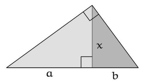
A geometric picture for the geometric mean starts with a right triangle. Lay it with its hypotenuse horizontal; then cut it with the altitude \(x\) into the light and dark subtriangles. The hypotenuse splits into two lengths \(a\) and \(b\), and the altitude \(x\) is their geometric mean \(\sqrt{ab}\).
Why is the altitude \(x\) equal to \(\sqrt{ab}\)?

To show that \(x = \sqrt{ab}\), compare the small, dark triangle to the large, light triangle by rotating the small triangle and laying it on the large triangle. The two triangles are similar! Therefore, their aspect ratios (the ratio of the short to the long side) are identical. In symbols, \(x/a = b/x\): The altitude x is therefore the geometric mean \(\sqrt{ab}\). The uncut right triangle represents the geometric-mean portion of the AM–GM inequality. The arithmetic mean \((a + b)/2\) also has a picture, as one-half of the hypotenuse. Thus, the inequality claims that
\[\frac{\text{ hypotenuse } }{2} \geqslant \text{ altitude } \label{4.15} \]
Alas, this claim is not pictorially obvious.
Can you find an alternative geometric interpretation of the arithmetic mean that makes the AM–GM inequality pictorially obvious?

The arithmetic mean is also the radius of a circle with diameter \(a + b\). Therefore, circumscribe a semicircle around the triangle, matching the circle’s diameter with the hypotenuse \(a + b\) (problem 4.7.). The altitude cannot exceed the radius; therefore,
\[\frac{a + b}{2} \geqslant \sqrt{ab} \label{4.16} \]
Furthermore, the two sides are equal only when the altitude of the triangle is also a radius of the semicircle namely when \(a = b\). The picture therefore contains the inequality and its equality condition in one easy- to-grasp object. (An alternative pictorial proof of the AM–GM inequality is developed in Problem 4.33.)
Problem 4.6 Circumscribing a circle around a triangle
Here are a few examples showing a circle circumscribed around a triangle.

Draw a picture to show that the circle is uniquely determined by the triangle.
Problem 4.7 Finding the right semicircle
A triangle uniquely determines its circumscribing circle (Problem 4.6). However, the circle’s diameter might not align with a side of the triangle. Can a semicircle always be circumscribed around a right triangle while aligning the circle’s diameter along the hypotenuse?
Problem 4.8 Geometric mean of three numbers
For three nonnegative numbers, the AM–GM inequality is
\[\frac{a + b + c}{3} \geqslant (abc)^{1/3}. \label{4.17} \]
Why is this inequality, in contrast to its two-number cousin, unlikely to have a geometric proof? (If you find a proof, let me know.)
Applications
Arithmetic and geometric means have wide mathematical application. The first application is a problem more often solved with derivatives: Fold a fixed length of fence into a rectangle enclosing the largest garden.
What shape of rectangle maximizes the area?

The problem involves two quantities: a perimeter that is fixed and an area to maximize. If the perimeter is related to the arithmetic mean and the area to the geometric mean, then the AM–GM inequality might help maximize the area. The perimeter \(P = 2(a + b)\) is four times the arithmetic mean, and the area \(A = ab\) is the square of the geometric mean. Therefore, from the AM–GM inequality,
\[\underbrace{\frac{P}{4}}_{\text{ AM }} \geqslant \underbrace{\sqrt{A}}_{\text{ GM }} \label{4.18} \]
with equality when \(a = b\). The left side is fixed by the amount of fence. Thus the right side, which varies depending on \(a\) and \(b\), has a maximum of \(P/4\) when \(a = b\). The maximal-area rectangle is a square.
Problem 4.9 Direct pictorial proof
The AM–GM reasoning for the maximal rectangular garden is indirect pictorial reasoning. It is symbolic reasoning built upon the pictorial proof for the AM– GM inequality. Can you draw a picture to show directly that the square is the optimal shape?
Problem 4.10 Three-part product
Find the maximum value of \(f(x) = x^{2}(1 − 2x)\) for \(x \geqslant 0\), without using calculus. Sketch \(f(x)\) to confirm your answer.
Problem 4.11 Unrestricted maximal area
If the garden need not be rectangular, what is the maximal-area shape?
Problem 4.12 Volume maximization
Build an open-topped box as follows: Start with a unit square, cut out four identical corners, and fold in the flaps.
The box has volume \(V = x(1 − 2x)^{2}\), where x is the side length of a corner cutout. What choice of x maximizes the volume of the box?

Here is a plausible analysis modeled on the analysis of the rectangular garden. Set \(a = x\), \(b = 1 − 2x\), and \(c = 1 − 2x\). Then abc is the volume V, and \(V^{1/3} = ^{3}\sqrt{abc}\) is the geometric mean (Problem 4.8). Because the geometric mean never exceeds the arithmetic mean and because the two means are equal when \(a = b = c\), the maximum volume is attained when \(x = 1 − 2x\). Therefore, choosing \(x = 1/3\) should maximize the volume of the box.
Now show that this choice is wrong by graphing \(V(x)\) or setting \(dV/dx = 0\); explain what is wrong with the preceding reasoning; and make a correct version.
Problem 4.13 Trigonometric minimum
Find the minimum value of
\[\frac{9x^{2} \sin^{2}x + 4}{x \sin x} \label{4.19} \]
in the region x \(\in\) (0, \(\pi\)).
Problem 4.14 Trigonometric maximum
In the region t \(\in\) [0, \(\pi/2\)], maximize \(\sin 2 t\) or, equivalently, 2 \(\sin t \cos t\).
The second application of arithmetic and geometric means is a modern, amazingly rapid method for computing \(\pi\) [5, 6]. Ancient methods for computing π included calculating the perimeter of many-sided regular polygons and provided a few decimal places of accuracy.
Recent computations have used Leibniz’s arctangent series
Imagine that you want to compute π to \(10^{9}\) digits, perhaps to test the hardware of a new supercomputer or to study whether the digits of π are random (a theme in Carl Sagan’s novel Contact [40]). Setting \(x = 1\) in the Leibniz series produces \(\pi/4\), but the series converges extremely slowly. Obtaining \(10^{9}\) digits requires roughly \(10^{10^{9}}\) terms—far more terms than atoms in the universe.
Fortunately, a surprising trigonometric identity due to John Machin (1686 – 1751) accelerates the convergence by reducing \(x\):
Even with the speedup, \(10^{9}\)-digit accuracy requires calculating roughly \(10^{9}\) terms.
In contrast, the modern Brent–Salamin algorithm [3, 41], which relies on arithmetic and geometric means, converges to π extremely rapidly. The algorithm is closely related to amazingly accurate methods for calculating the perimeter of an ellipse (Problem 4.15) and also for calculating mutual inductance [23]. The algorithm generates several sequences by starting with \(a_{0}\) = 1 and \(g_{0}\) = 1/\(\sqrt{2}\); it then computes successive arithmetic means \(a_{n}\), geometric means \(g_{n}\), and their squared differences \(d_{n}\).
\[a_{n+1}=\frac{a_{n}+g_{n}}{2}, \quad g_{n+1}=\sqrt{a_{n} g_{n}}, \quad d_{n}=a_{n}^{2}-g_{n}^{2} \label{4.23} \]
The a and g sequences rapidly converge to a number M(\(a_{0}\), \(g_{0}\)) called the arithmetic–geometric mean of \(a_{0}\) and \(g_{0}\). Then M(\(a_{0}\), \(g_{0}\)) and the difference sequence d determine π.
\[\pi=\frac{4 M\left(a_{0}, g_{0}\right)^{2}}{1-\sum_{j=1}^{\infty} 2^{j+1} d_{j}} \label{4.24} \]
The d sequence approaches zero quadratically; in other words, \(d_{n+1}\) ∼ \(d^{2}_{n}\) (Problem 4.16). Therefore, each iteration in this computation of π doubles the digits of accuracy. A billion-digit calculation of π requires only about 30 iterations far fewer than the 10109 terms using the arctangent series with \(x = 1\) or even than the \(10^{9}\) terms using Machin’s speedup.
Problem 4.15 Perimeter of an ellipse
To compute the perimeter of an ellipse with semimajor axis \(a_{0}\) and semiminor axis \(g_{0}\), compute the a, g, and d sequences and the common limit M(\(a_{0}, g_{0})\) of the a and g sequences, as for the computation of \(\pi\). Then the perimeter P can be computed with the following formula:
\[P=\frac{A}{M\left(a_{0}, g_{0}\right)}\left(a_{0}^{2}-B \sum_{j=0}^{\infty} 2^{j} d_{j}\right)\label{4.25} \]
where A and B are constants for you to determine. Use the method of easy cases (Chapter 2) to determine their values. (See [3] to check your values and for a proof of the completed formula.)
Problem 4.16 Quadratic convergence
Start with \(a_{0} = 1\) and \(g_{0} = 1/\sqrt{2}\) (or any other positive pair) and follow several iterations of the AM–GM sequence
\[a_{n + 1} = \frac{a_{n}+ g_{n}}{2} \text{ and } g_{n + 1} = \sqrt{a_{n}g_{n}}. \label{4.26} \]
Then generate \(d_{n} = a^{2}n − g^{2}n\) and \(log_{10}\) dn to check that \(d_{n+1} ∼ d^{2}_{n}\) (quadratic convergence).
Problem 4.17 Rapidity of convergence
Pick a positive \(x_{0}\); then generate a sequence by the iteration
\[x_{n + 1} = \frac{1}{2}(x_{n} + \frac{2}{x_{n}}) (n \geqslant 0) \label{4.27} \]
To what and how rapidly does the sequence converge? What if \(x_{0} < 0\)?